From SELECT to Advanced SQL: JOINs, CTEs, and More

SQL is one of the very few technologies in software engineering that does not fade with trends.

Frameworks change every few years. Backend stacks rotate. Frontend ecosystems reinvent themselves. But SQL stays.

That is not nostalgia. That is infrastructure.

SQL became the universal language of data. Whether a team uses PostgreSQL, MySQL, ClickHouse, Snowflake, or something distributed and exotic --- chances are, they still speak SQL.

Understanding SQL today is not optional for serious developers.

Backend engineers need it to avoid pushing database logic into application code. Analysts rely on it daily. QA engineers use it to validate system state. Product managers use it to inspect metrics without waiting for analytics pipelines.

This article walks through SQL step by step --- from simple SELECT queries to advanced window functions --- using practical examples and a PostgreSQL‑friendly syntax.

1. Database Anatomy: What We Actually Work With

Before writing queries, it helps to understand what the database really is.

A relational database is simply structured tables connected by rules. Think of it as Excel with strict discipline — no messy types, no broken references, no silent mistakes.

Each table contains:

• Columns (structure)
• Rows (actual data)

The power comes from constraints and relationships.

Unlike spreadsheets, relational databases enforce:

1. Strong typing
2. Explicit relationships

Primary Keys and Foreign Keys

Primary Key (PK) --- unique row identifier.

Foreign Key (FK) --- reference to another table’s primary key.

Example:

• users(id, name)
• orders(id, user_id, total)

orders.user_id references users.id.

This guarantees consistency: the database will reject an order for a non‑existent user.

Common Data Types

Most projects rely on a core set:

• INT / BIGINT --- numeric identifiers and counters
• TEXT / VARCHAR --- strings
• TIMESTAMPTZ --- date-time stored in UTC
• JSONB (PostgreSQL) --- flexible semi‑structured data

Always store timestamps in UTC. Convert on the client side.

2. Reading Data: SELECT

The most common SQL operation is reading.

Basic query:

SELECT name, price
FROM products;

Avoid:

SELECT *
FROM products;

Why? Because production systems scale. Fetching unnecessary columns wastes bandwidth, memory, and sometimes performance advantages from indexes.

Aliases

SELECT
  name AS product_name,
  price AS product_price
FROM products;

This is especially helpful in complex JOIN queries.

DISTINCT

Use DISTINCT when you care about unique values, not raw rows.

SELECT DISTINCT category
FROM products;

Pagination

SELECT id, name
FROM products
ORDER BY id
LIMIT 10 OFFSET 20;

Large OFFSET values are inefficient. Prefer keyset pagination in high‑load systems:

SELECT id, name
FROM products
WHERE id > 1000
ORDER BY id
LIMIT 10;

OFFSET works for small pages. For large datasets, keyset pagination is more efficient.

3. Filtering and Sorting

Filtering uses WHERE.

Filtering narrows data down to what actually matters.

Instead of loading everything and filtering in application code, push logic into the database — it is optimized for this.

SELECT name, price
FROM products
WHERE category = 'phones'
  AND price > 50000;

IN

Cleaner than multiple OR statements.

WHERE category IN ('phones', 'laptops')

BETWEEN

Readable range filter.

WHERE price BETWEEN 30000 AND 60000

LIKE / ILIKE

Pattern matching for text.

WHERE name LIKE 'iPhone%'

Postgres case-insensitive:

WHERE name ILIKE 'iphone%'

NULL Handling

NULL means “unknown”, not empty.

Incorrect:

WHERE description = NULL

Correct:

WHERE description IS NULL

ORDER BY

Sorting is expensive on large datasets — especially without indexes.

SELECT name, price
FROM products
ORDER BY price DESC, name ASC;

Sorting large datasets without indexes is expensive.

4. Aggregation and GROUP BY

Aggregation turns raw data into insight.

Instead of looking at thousands of rows, we compute metrics.

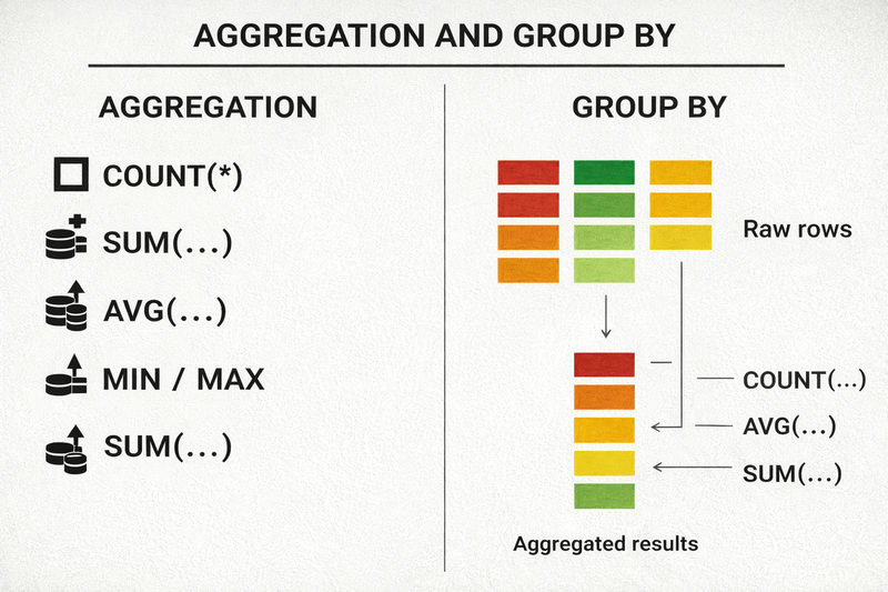
Aggregate functions:

• COUNT
• SUM
• AVG
• MIN
• MAX

Example:

SELECT
  MAX(price) AS max_price,
  AVG(price) AS avg_price,
  COUNT(*) AS total_products
FROM products;

GROUP BY

Grouping splits rows into logical buckets before aggregation.

SELECT
  category,
  COUNT(*) AS product_count,
  AVG(price) AS avg_price
FROM products
GROUP BY category;

Rule:

Every non-aggregated column in SELECT must appear in GROUP BY.

HAVING

HAVING filters groups after aggregation — unlike WHERE.

Incorrect:

SELECT category, COUNT(*)
FROM products
WHERE COUNT(*) > 10
GROUP BY category;

Correct:

SELECT category, COUNT(*)
FROM products
GROUP BY category
HAVING COUNT(*) > 10;

5. JOINs

Real SQL begins with JOINs.

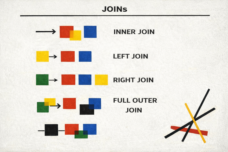
JOINs connect tables. This is where relational databases shine.

Instead of duplicating data, we combine normalized structures dynamically.

INNER JOIN

SELECT u.name, o.total
FROM users u
JOIN orders o ON u.id = o.user_id;

Only matching rows are returned.

LEFT JOIN

SELECT u.name, o.total
FROM users u
LEFT JOIN orders o ON u.id = o.user_id;

All users appear. Missing matches become NULL.

Find users without orders:

SELECT u.name
FROM users u
LEFT JOIN orders o ON u.id = o.user_id
WHERE o.id IS NULL;

SELF JOIN

Used when a table references itself (hierarchies, managers, categories).

SELECT e.name AS employee,
       m.name AS manager
FROM employees e
LEFT JOIN employees m ON e.manager_id = m.id;

6. Data Modification (DML)

These queries change actual data.

Use carefully.

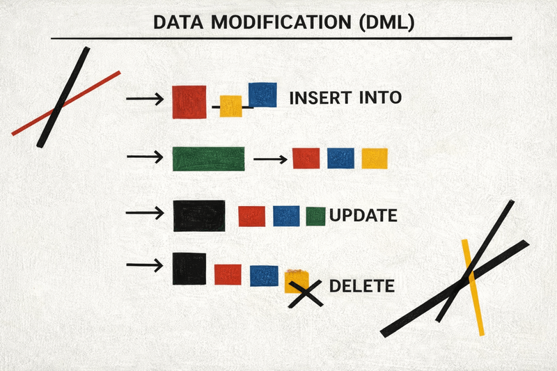
INSERT

INSERT INTO users (name, email)
VALUES ('Alex', 'alex@example.com');

Always list columns.

UPDATE

UPDATE products
SET price = 65000
WHERE id = 42;

Never run UPDATE without WHERE unless intentional.

DELETE

DELETE FROM users
WHERE last_login < '2020-01-01';

TRUNCATE

TRUNCATE TABLE logs;

Instantly removes all rows.

7. Schema Changes (DDL)

DDL modifies structure, not data.

Think of it as plumbing — not water.

CREATE TABLE

Defines structure and constraints.

CREATE TABLE orders (
  id BIGSERIAL PRIMARY KEY,
  user_id BIGINT NOT NULL,
  total NUMERIC(10,2) DEFAULT 0,
  created_at TIMESTAMPTZ DEFAULT NOW()
);

ALTER TABLE

Adds or modifies columns safely.

ALTER TABLE orders
ADD COLUMN promo_code TEXT;

DROP TABLE

DROP TABLE orders;

Removes table permanently.

DDL is powerful and dangerous — migrations exist for a reason. Use with extreme caution!

8. Subqueries and CTE

When logic becomes complex, structure matters.

Subquery

Subqueries embed logic inline.

SELECT name, salary
FROM employees
WHERE salary > (
  SELECT AVG(salary) FROM employees
);

CTE

CTEs (WITH) make queries readable and modular. They allow you to break large queries into understandable blocks.

WITH top_customers AS (
  SELECT user_id, SUM(total) AS spent
  FROM orders
  GROUP BY user_id
  HAVING SUM(total) > 100000
)
SELECT *
FROM top_customers;

CTEs improve readability.

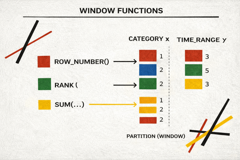
9. Window Functions

Window functions compute aggregates without collapsing rows.

Example: top 3 salaries per department.

WITH ranked AS (
  SELECT
    department,
    name,
    salary,
    RANK() OVER (
      PARTITION BY department
      ORDER BY salary DESC
    ) AS dept_rank
  FROM employees
)
SELECT *
FROM ranked
WHERE dept_rank <= 3;

Window functions enable:

• Ranking
• Running totals
• Moving averages
• Row comparisons (LAG / LEAD)

Once mastered, window functions replace large portions of application-side logic.

10. Logical Execution Order

SQL executes in this order:

1. FROM / JOIN
2. WHERE
3. GROUP BY
4. HAVING
5. SELECT
6. ORDER BY
7. LIMIT

Understanding this prevents common mistakes.

11. Indexes and Performance

Indexes allow fast lookups.

Example:

SELECT id, status
FROM users
WHERE status = 'VIP';

If index covers these columns, database can avoid reading full rows.

But:

SELECT *
FROM users
WHERE status = 'VIP';

Forces table fetches.

Always select only required columns.

Conclusion

SQL is easy to start and difficult to master.

Core recommendations:

• Avoid SELECT *
• Use LEFT JOIN intentionally
• Understand NULL
• Learn window functions early
• Know execution order

Frameworks change. Data remains.

Invest in SQL.